Tree types
“Tree” is broad: this page groups binary tree shapes, search-tree families, heaps, advanced structures (B-tree, trie, …), and special variants. Definitions vary by textbook—match your course’s wording before exams.
- What is a tree, general tree, and binary tree (with figure)
- General vs binary (summary table)
- Binary tree shapes: full, complete, perfect, balanced, degenerate
- BST family: BST, AVL, red–black, splay
- Heaps; advanced trees; special trees
1) What is a tree?
In data structures, a tree is a hierarchical collection of nodes joined by edges. It has exactly one root (the node with no parent); every other node has exactly one parent. Trees are acyclic: there is only one simple path between any two nodes. This shape models file folders, org charts, syntax of expressions, game moves, and many recursive algorithms.
2) What is a general tree?
A general tree (also called an N-ary tree) does not limit how many children a node may have—each node can have zero or more ordered or unordered children depending on the problem. Implementation options include arrays of child pointers, linked lists of children, or the classic first-child / next-sibling representation (which uses a binary-tree–shaped overlay to store an arbitrary tree).
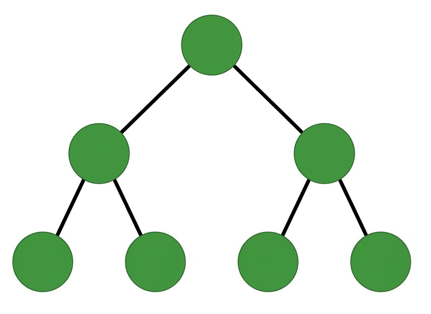
3) What is a binary tree?
A binary tree is a tree in which each node has at most two children, usually distinguished as left and right. Missing children are represented as absent links (NULL in C). Binary trees are the usual starting point for heaps, BSTs, and segment-tree ideas in coursework.
4) General vs binary
| Type | Rule | Notes |
|---|---|---|
| General (N-ary) tree | Each node may have any number of children. | Often stored as “first child / next sibling” or list of children. |
| Binary tree | Each node has at most two children: left and right. | Missing child = NULL in pointer-based C. |
5) Types of binary trees (shape & structure)
These classify shape only (no key ordering unless stated).
Full binary tree
Every internal node has exactly two children; leaves have zero. Equivalently: no node with exactly one child. (Some books misuse “full” for “complete”—check your syllabus.)
Example: a small full tree (only 0- or 2-child nodes):
       o
     /   \
    o     o
   / \   / \
  o   o o   o
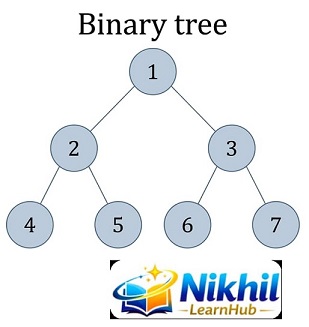
Complete binary tree
All levels are completely filled except possibly the last, and the last level is filled from left to right with no gaps. This is the shape used by binary heaps in arrays (parent at i, children at 2i+1, 2i+2).
Example: 7 nodes packed left-to-last level:
        1
      /   \
     2     3
    / \   /
   4   5 6
Perfect binary tree
Every internal node has two children and all leaves share the same depth. For height h (edges from root to deepest leaf), node count is 2h+1 − 1 with the usual conventions.
Example: height 2, 7 nodes:
        o
      /   \
     o     o
    / \   / \
   o   o o   o
Balanced binary tree
Height is kept small (often O(log n)) relative to the number of nodes—typically by rotation or color rules—so search and update stay efficient. AVL and red–black trees are common balanced BSTs.
Example: inserting sorted keys 1,2,3,4,5 into a plain BST gives a tall chain; a balanced policy reshapes so depth stays logarithmic.
Degenerate (skewed) binary tree
Each node has at most one child— the tree collapses to a linked-list shape. Worst case for unbalanced BST insert of sorted data: height n−1, search becomes O(n).
Example: only right children (keys inserted in order):
1
 \
  2
   \
    3
     \
      4
6) Binary search trees (BST family)
All are binary trees plus ordering (and often extra invariants). Typical rule: left < root < right for comparable keys (define ties explicitly).
Binary search tree (BST)
For every node, all keys in the left subtree are less than the node’s key and all keys in the right subtree are greater. Enables inorder walk in sorted order and guided search.
Example: keys 5, 3, 7, 1, 4:
      5
    /   \
   3     7
  / \
 1   4
AVL tree
A self-balancing BST: for every node, the height of the left and right subtrees differs by at most 1. Inserts/deletes may trigger rotations to restore balance. Guarantees O(log n) search in the worst case.
Example: after inserting 1,2,3 in order, an AVL rotates so the root is 2, not a skewed chain.
Red–black tree
A balanced BST using node colors (red/black) and rules (e.g. no two consecutive red edges, black depth same for all leaves). Slightly looser than AVL but fewer rotations on average—used in many libraries (e.g. C++ std::map, Linux kernel rbtree).
Example: same keys as a BST, but recolor/rotate after insert to keep black-height balanced.
Splay tree
A self-adjusting BST: accessing a node splays it to the root with rotations. Recently used keys stay near the top—good for locality (cache-like behavior); amortized O(log n) per operation.
Example: repeated searches for key 42 make 42 bubble up toward the root over time.
7) Heap trees
A binary heap is usually a complete binary tree stored in an array, with a heap order property.
| Kind | Property | Example use |
|---|---|---|
| Min-heap | Parent key ≤ both children (recursively). Smallest at root. | Priority queue “take smallest”, Dijkstra with heaps. |
| Max-heap | Parent key ≥ both children. Largest at root. | Heap sort (ascending build from max-heap), priority “take largest”. |
Example (min-heap of values): root is minimum; shape is complete.
        2
      /   \
     5     3
    / \   /
   9   6 4
Used in: priority queues, heap sort, graph algorithms (shortest paths), and scheduling. This tutorial’s C focus: see priority queue (heap) when you connect heaps to code.
8) Advanced trees
Brief reference; full implementations are usually beyond a first C DS course.
B-tree
Generalization of BST for disk: nodes hold many keys and children, height stays low to reduce I/O. Used in databases and file systems.
Example: a database index on “user_id” stored as a B-tree so each disk page holds a range of keys.
B+ tree
Like a B-tree, but data records live only in leaves; internal nodes are pure keys for navigation. Leaves are often linked for range scans. Common in MySQL InnoDB and many DB indexes.
Example: SQL WHERE id BETWEEN 100 AND 200 walks the B+ leaf chain.
Trie (prefix tree)
Edges labeled with characters; paths from the root spell strings. Great for prefix search, autocomplete, and XOR basis problems (bit tries).
Example: store cat, car, card—shared prefix ca appears once.
Segment tree
Binary tree over an array segment; each node stores an aggregate (sum, min, …) for its range. Supports range queries and updates in O(log n) with lazy propagation when needed.
Example: array [2,5,1,4]—root holds sum 12; children hold sums of halves.
Fenwick tree (Binary Indexed Tree)
Flat array structure (not always drawn as a tree) that supports prefix sums and point updates in O(log n). Simpler to code than segment trees for pure prefix problems.
Example: frequency table of values—add to index i, query sum from 1 to i.
Suffix tree
Compresses all suffixes of a string into a tree (or array + LCP) for fast substring and pattern queries—classic in bioinformatics and competitive programming (often paired with suffix arrays).
Example: find if ana occurs in banana by walking from the root following edge labels.
9) Special trees
N-ary tree
Each node may have up to N children (general tree). Examples: parse trees with variable arity, organizational charts, UI component trees with many branches.
Example: file system—folder “Documents” has many subfolders without a fixed binary split.
Threaded binary tree
Unused NULL child pointers are replaced by threads to inorder predecessor/successor so you can traverse without a stack or recursion—useful for iterative inorder on memory-tight systems.
Example: after threading, “next” from the leftmost node follows threads instead of an explicit parent stack.
Expression tree
Leaves are operands; internal nodes are operators. Evaluating postorder = RPN evaluation; inorder with parentheses shows the infix expression.
Example: (3 + 4) * 5 as a tree with * at root, + as left child of *, and 5 as right child—see Expression tree (stack).
C implementations in this track start with representation, then binary tree operations, binary tree (array), linked list, BST, plus AVL, red-black, B-tree, and B+ tree overviews.
Key takeaway
Separate shape (full/complete/perfect/skewed), ordering (BST family), and application (heap, trie, B-tree). Pick the minimal structure that matches your access pattern and complexity needs.
Next up: Tree traversal methods · Tree representation · Binary tree operations